Postprocessing

The postprocessing stage of a script processes the data from a finished simulation, for example plotting or exporting the value of the subjects’ state variables (v-values or w-values).

The postprocessing commands are the following:

Command	Description	Affected by parameters
@figure	Creates a figure window	None
@subplot	Creates a subplot within the current figure window	None
@legend	Creates a legend for all plotted lines in the current subplot	None
@vplot	Plots a v-value	runlabel, xscale, xscale_match, phases, subject
@vssplot	Plots a vss-value (only in the Rescorla-Wagner mechanism	runlabel, xscale, xscale_match, phases, subject
@pplot	Plots the probabilitiy to respond with a certain behavior to a certain stimulus	runlabel, xscale, xscale_match, phases, subject
@wplot	Plots a w-value	runlabel, xscale, xscale_match, phases, subject
@nplot	Plots the number of occurrences of a certain stimulus/behavior or a chain stimulus->behavior->stimulus->... or behavior->stimulus->behavior->...	runlabel, xscale, xscale_match, phases, subject, cumulative, match
@vexport	Exports the values of a @vplot	filename and same as @vplot
@vssexport	Exports the values of a @vssplot	filename and same as @vssplot
@pexport	Exports the values of a @pplot	filename and same as @pplot
@wexport	Exports the values of a @wplot	filename and same as @wplot
@nexport	Exports the values of a @nplot	filename and same as @nplot
@hexport	Exports the history of stimuli and responses	filename, runlabel

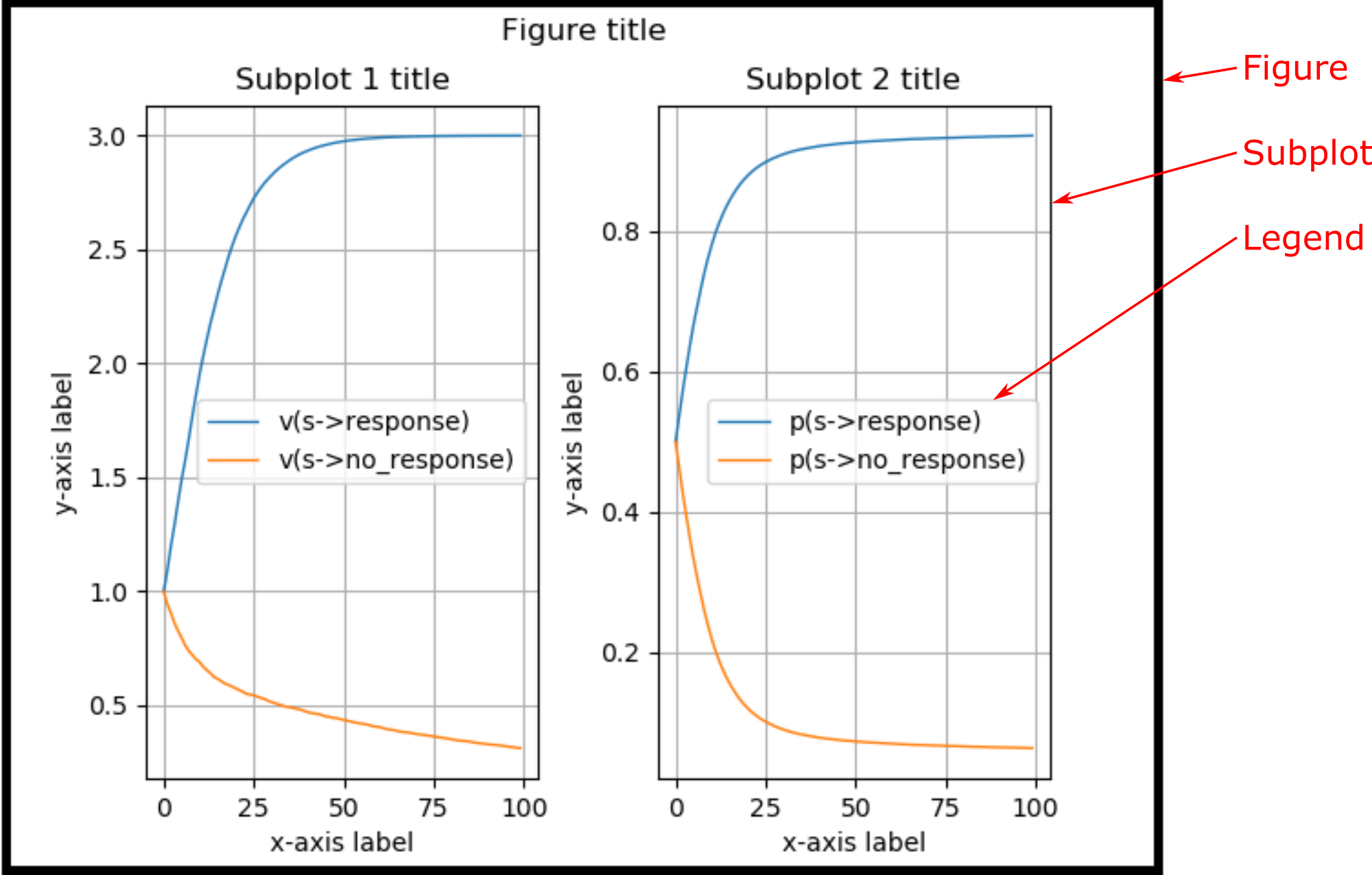
The below plots show the components of a plot window:

@figure

Creates a new figure window.

Syntax:

@figure
@figure figure_title
@figure figure_title figure_parameters
@figure figure_parameters

where

• figure_title is an optional title of the figure (any string),

• figure_parameters is an optional specification of Matplotlib Figure parameters controlling figure size, colors, etc. of the format {param1:value1, param2:value2, ...}. See figure_parameters for the supported figure parameters.

Note

If a plot command or a @subplot command is issued without a preceding @figure command, a default figure window will automatically be created.

Example 1

@figure

creates a default figure without title and with the default Matplotlib Figure parameters.

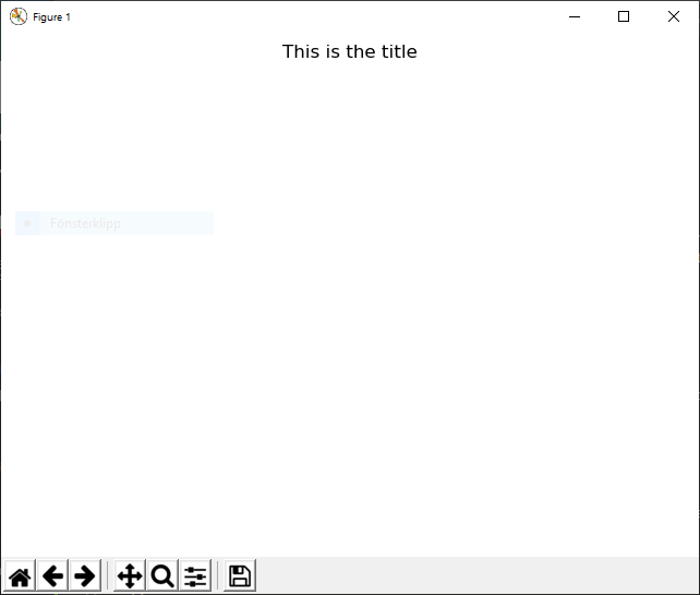
Example 2

@figure This is the title

creates a figure with the title “This is the title” and with the default Matplotlib Figure parameters:

Example 3

@figure This is the title {'edgecolor':'blue','linewidth':10,'facecolor':'red'}

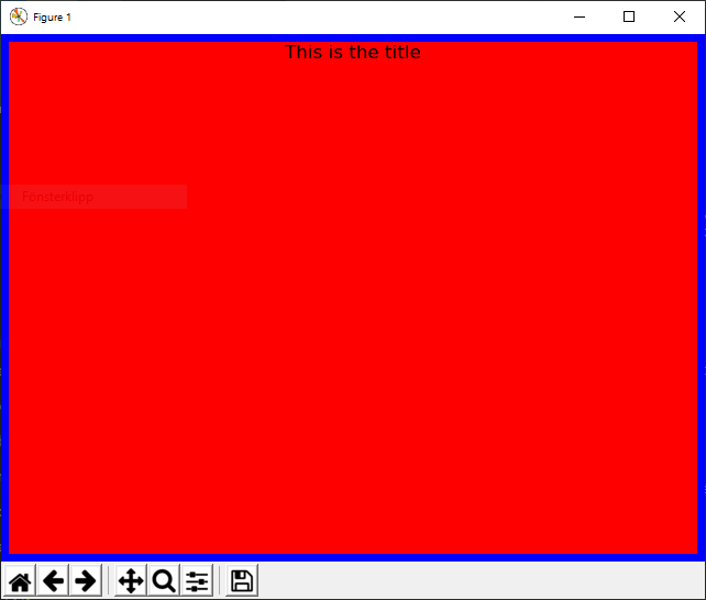
creates a figure with the title “This is the title” with a blue edge (width 10) and red background:

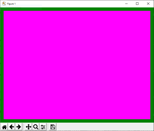
Example 4

@figure {'edgecolor':'green','linewidth':20,'facecolor':'magenta'}

creates a figure without title and with a green edge (width 5) and magenta background:

@subplot

The command @subplot creates an axis within a figure in which to make plots using any of the plotting commands (@vplot, @wplot, etc.)

Syntax:

@subplot pos
@subplot pos subplot_title
@subplot pos subplot_title subplot_parameters

• pos describes the position of the subplot within the figure. It is either a 3-digit integer (nrows)(ncols)(index) (for example 223), or three comma-separated integers in parenthesis (nrows, ncols, index) (for example (2,2,3)). The subplot will take the position index on a grid with nrows rows and ncols columns. index starts at 1 in the upper left corner and increases to the right.

• subplot_parameters is an optional specification of Matplotlib Subplot parameters controlling for example the background color, in the format {param1:value1, param2:value2, ...}. See subplot parameters for the supported subplot parameters.

Useful Subplot parameters to control the appearance of the subplot include

• xlim (The min- and max value of the x-axis)

• ylim (The min- and max value of the y-axis)

• xlabel (The label of the x-axis)

• ylabel (The label of the y-axis)

stated as:

{'xlim':[xmin,xmax], 'ylim':[ymin,ymax], 'xlabel':'x-axis label', 'ylabel':'y-axis label'}

where xmin, xmax, ymin, and ymax are numbers.

Note

If a plot command is issued without a preceding @subplot command, a default subplot axis will automatically be created (corresponding to @subplot 111).

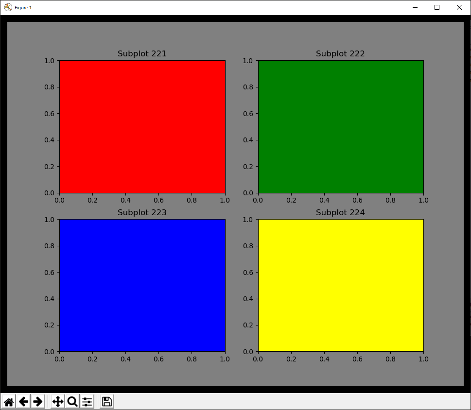
Example

@figure {'edgecolor':'black','linewidth':20,'facecolor':'grey'}
@subplot 221 Subplot 221 {'facecolor':'red'}
@subplot 222 Subplot 222 {'facecolor':'green'}
@subplot 223 Subplot 223 {'facecolor':'blue'}
@subplot 224 Subplot 224 {'facecolor':'yellow'}

@legend

The command @legend creates a legend with labels for each plotted curve in the last created subplot. For the labels, the legend uses default descriptive labels (that depends on the type of plot), but these may be overridden by custom labels using the label parameter to the plotting commands.

Syntax:

@legend
@legend legend_parameters

where legend_parameters is an optional specification of Matplotlib Legend parameters controlling for example the frame and background colors, in the format {param1:value1, param2:value2, ...}. See legend parameters for the supported legend parameters.

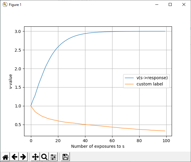
Example 1

Running this script:

n_subjects        = 100
mechanism         = sr
behaviors         = response, no_response
stimulus_elements = background, s, reward
start_v           = default:1
alpha_v           = 0.1
u                 = reward:3, default:0

@PHASE training stop: s==100
START_TRIAL s          | response: REWARD | NO_REWARD
REWARD      reward     | START_TRIAL
NO_REWARD   background | START_TRIAL

@run training

xscale = s

# Postprocessing commands
@subplot 111 {'xlabel':'Number of exposures to s', 'ylabel':'v-value'}
@vplot s->response
@vplot s->no_response {'label':'custom label'}
@legend

creates the following plot:

Example 2

With the same simulation as in Example 1 but the following postprocessing commands:

@vplot s->response {'linestyle':'--', 'color':'black'}
@vplot s->no_response {'label':'my custom label', 'marker':'o', 'color':'red','markevery':10}
@legend {'title':'my legend title', 'fontsize':20, 'facecolor':'grey'}

creates the following figure:

@vplot

The command @vplot plots a v-value (the associative strength between a stimulus element and a behavior).

Syntax:

@vplot e->b
@vplot e->b line_parameters

plots the associative strength between the stimulus element e and the behavior b, and line_parameters are Line2D parameters.

@vssplot

The command @vssplot plots a vss-value (the associative strength between two stimulus elements).

Note

Only the Rescorla-Wagner learning mechanism has vss-values, so the command @vssplot is only applicable when mechnism=rw.

Syntax:

@vssplot e1->e2
@vssplot e1->e2 line_parameters

plots the associative strength between the stimulus elements e1 and e2, and line_parameters are Line2D parameters.

@pplot

The command @pplot plots the probability of responding with a certain behavior to a certain stimulus, according to The decision function.

Syntax:

@pplot s->b
@pplot s->b line_parameters

plots the probability of responding with b to the stimulus s, and line_parameters are Line2D parameters.

@wplot

The command @wplot plots a w-value (the conditioned reinforcement for a stimulus element) for the mechanisms that support this (Guided associative learning and Actor-critic).

Syntax:

@wplot e
@wplot e line_parameters

plots the conditioned reinforcement value for the stimulus element e, and line_parameters are Line2D parameters.

@nplot

The command @nplot plots the number of occurrences of a stimulus, a behavior, or a chain stimulus->behavior->stimulus->... or behavior->stimulus->behavior->... in the history of stimulus-response pairs during the simulation, and line_parameters are Line2D parameters.

Syntax:

@nplot stimulus
@nplot behavior
@nplot stimulus1->behavior1->stimulus2->...
@nplot behavior1->stimulus1->behavior2->...
@nplot ... line_parameters

where stimulus is a stimulus, i.e. in general a comma-separated list of stimulus elements, behavior is a behavior, and line_parameters are Line2D parameters.

cumulative

The parameter cumulative can have the values on or off and affects @nplot input in the following way:

If cumulative is off:

• If xscale is all: At each point (stimulus or response) in the history, the y-value is 1 if input matches the simulation sequence at that point, and 0 otherwise.

• If xscale is not all: The y-value shows the number of occurrences of input between each point (stimulus or response) in the history where xscale matches the simulation sequence. For example, the y-value at \(x=1\) is the number of occurrences of input between the first and the second occurrence of input, and the y-value at \(x=2\) is the number of occurrences of input between the second and the third, etc.

If cumulative is on, the values above are added cumulatively at each x-value. For example, the value at \(x=4\) shows the sum of the values at \(x=0\), \(x=1\), \(x=2\), and \(x=3\).

Note

With multiple subjects and subject=average the plotting commands (including @nplot) renders the average y-value of all subjects, which means that the y-value can be between 0 and 1 even if the y-value for each individual subject is 0 or 1.

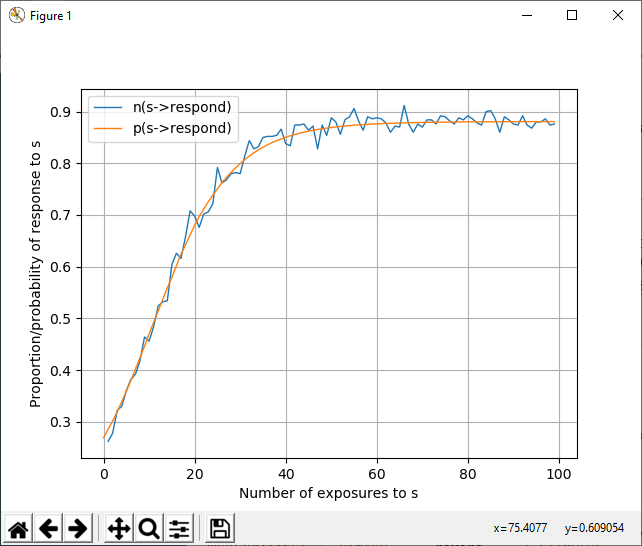
Example

With the combination xscale=s (for some stimulus s), cumulative=off, and n_subjects>1:

@pplot s->b

shows, at each exposure of s, the probability to respond with the behavior b to the stimulus s, whereas:

@nplot s->b

shows, at each exposure of s, the empirical average (over all subjects) fraction of times when an subject responded with b to s in the simulation:

n_subjects        = 500
mechanism         = SR
behaviors         = respond,ignore
stimulus_elements = s, reward
start_v           = s->ignore:0, default:-1
alpha_v           = 0.1
beta              = 1
u                 = reward:2, default:0

@phase instrumental_conditioning stop:s=100
STIMULUS    s          | respond: REWARD  | STIMULUS
REWARD      reward     | STIMULUS

@run instrumental_conditioning

xscale     = s
cumulative = off

@subplot 111 {'xlabel':'Number of exposures to s', 'ylabel':'Proportion/probability of response to s'}
@nplot s->respond
@pplot s->respond
@legend

Line2D parameters

The input line_parameters to the plotting commands is an optional specification of Matplotlib Line2D parameters controlling for example line color and line style, in the format {param1:value1, param2:value2, ...}. See Line2D parameters for the supported Line2D parameters.

Use the Line2D parameter label to set a custom label for the legend (produced with @legend) to the plotted line.

Useful Line2D parameters to control the appearance of the plot include color, linestyle, marker, markevery.

Exporting data to file

The data-exporting commands @vexport, @wexport, @pexport, and @nexport exports to a csv-file the data that is plotted with the plotting commads @vplot, @wplot, @pplot, and @nplot, respectively. Therefore the same parameters that affect the plot also affect the exported data (for example xscale, phases, subject, runlabel, etc.)

In addition, the parameter filename is required to all exporting commands.

The command @hexport simply exports the sequence of alternating stimuli and responses for the @run specified with the parameter runlabel. There is one sequence for each subject (regardless of the value of the parameter subject). The exported data with @hexport is not affected by any other parameter.

The destination file is specified with the parameter filename.

Note

If the specified file already exists, the existing file will be overwritten without warning.

Format of the csv-file

The data export commands @vexport, @wexport, @pexport, and @nexport exports the data as a csv-file with two or more columns. The first column, with title “x” contains step numbers (corresponding to the x-axis in the corresponding plot command). The second column onwards contains the data for the specified quantity for each subject (controlled by the subject parameter). For example, after the commands:

n_subjects = 5
subject = all
filename = my_file.csv
@vexport s->b

the first line, containing the headings, in the file my_file.csv looks like this:

"x","v(s->b) subject 0","v(s->b) subject 1","v(s->b) subject 2","v(s->b) subject 3","v(s->b) subject 4"

If instead subject = average, the first line will look like this:

"x","v(s->b)"

The remaining lines contain comma-separated values for the quantities in the heading. An example csv-file exported with @vexport s->response may look like this:

"x","v(s->response) subject 0","v(s->response) subject 1","v(s->response) subject 2","v(s->response) subject 3","v(s->response) subject 4"
0,1,1,1,1,1
1,1.2,1.2,1.2,1,1
2,1.2,1.2,1.2,1,1
3,1.38,1.2,1.38,1.2,1.2
4,1.38,1.2,1.38,1.2,1.2
5,1.38,1.38,1.5419999999999998,1.38,1.2
6,1.38,1.38,1.5419999999999998,1.38,1.2
7,1.5419999999999998,1.38,1.6877999999999997,1.38,1.38
8,1.5419999999999998,1.38,1.6877999999999997,1.38,1.38
9,1.6877999999999997,1.5419999999999998,1.8190199999999999,1.5419999999999998,1.38

The @hexport command exports the sequence of alternating stimuli and responses for each subject, and has therefore a different format. See @hexport.

@vexport

@vexport exports the data plotted by @vplot to the csv-file specified with the parameter filename.

Syntax:

filename = my_file.csv
@vexport e->b

See also Format of the csv-file.

@vssexport

@vssexport exports the data plotted by @vssplot to the csv-file specified with the parameter filename.

Note

Only the Rescorla-Wagner learning mechanism has vss-values, so the command @vssplot is only applicable when mechnism=rw.

Syntax:

filename = my_file.csv
@vssexport e1->e2

See also Format of the csv-file.

@pexport

@pexport exports the data plotted by @pplot to the csv-file specified with the parameter filename.

Syntax:

filename = my_file.csv
@pexport s->b

See also Format of the csv-file.

@wexport

@wexport exports the data plotted by @wplot to the csv-file specified with the parameter filename.

Syntax:

filename = my_file.csv
@vexport e

See also Format of the csv-file.

@nexport

@nexport exports the data plotted by @nplot to the csv-file specified with the parameter filename.

Syntax:

filename = my_file.csv
@nexport stimulus
@nexport behavior
@nexport stimulus1->behavior1->stimulus2->...
@nexport behavior1->stimulus1->behavior2->...

See also Format of the csv-file.

@hexport

The @hexport command exports a csv-file with three or more columns. Column 1 contains step numbers. Columns 2 and 3 contains the stimulus and response, respectively, for subject 1. Column 4 and 5 contains the stimulus and response, respectively, for subject 2, etc:

"step","stimulus subject 0","response subject 0","stimulus subject 1","response subject 1","stimulus subject 2","response subject 2",...

Note

All subjects are always included in the output file from @hexport.